The LM Curve. For the LM curve, the independent variable is income and the dependent variable is the interest rate.

For the LM curve, the independent variable is income and the dependent variable is the interest rate.

The LM curve shows the combinations of interest rates and levels of real income for which the money market is in equilibrium. The initials LM stand for " Liquidity preference and Money supply equilibrium".

Two basic elements determine the quantity of cash balances demanded (liquidity preference) and therefore the position and slope of the function:

1. Transactions demand for money: this includes both the willingness to hold cash for everyday transactions and a precautionary measure (money demand in case of emergencies). Transactions demand is positively related to real GDP. This is simply explained - as GDP increases, so does spending and therefore transactions.

2. Speculative demand for money: this is the willingness to hold cash instead of securities as an asset for investment purposes. Speculative demand is inversely related to the interest rate.

The money supply is determined by the central bank decisions and willingness of commercial banks to loan money.

Mathematically, the LM curve is defined by the equation

M/P = L(i, Y)

where the supply of money is represented as the real amount M/P (as opposed to the nominal amount M), with P representing the price level, and L being the real demand for money, which is some function of the interest rate i and the level Y of real income.The LM curve shows the combinations of interest rates and levels of real income for which money supply equals money demand — that is, for which the money market is in equilibrium.

The LM curve is upward sloping because higher income results in higher demand for money, thus resulting in higher interest rates.The intersection of the IS curve with the LM curve shows the equilibrium interest rate and price level.

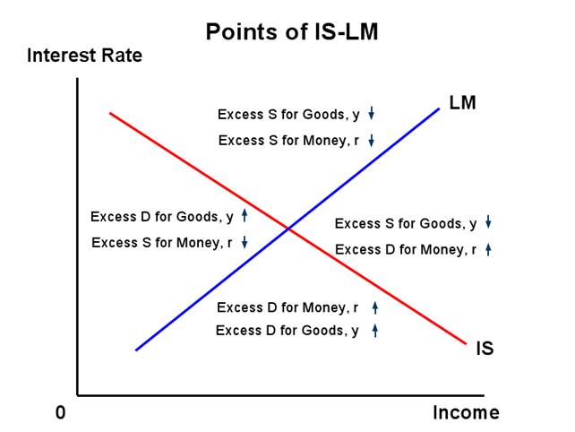
3. Shifts, Points of The IS-LM Model & Incorporation Into Larger Models

The IS curve and the LM curve shift in response to economic activities.

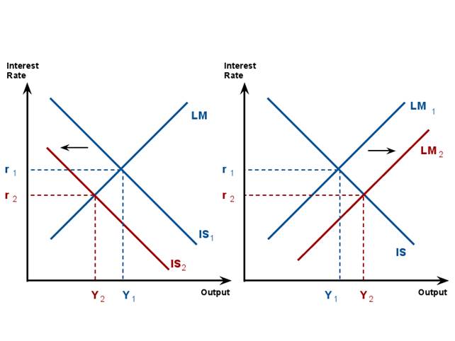
The IS curve shifts outward as a result of increased government purchases, exogenous increases in investment, decreases in taxes, and exogenous increases in consumption, and vice versa.

The LM curve shifts outward as a result of increases in the money supply and decreases in the price level, and vice versa.

By itself, the IS-LM model is used to study the short run when prices are fixed or sticky and no inflation is taken into consideration. But in practice the main role of the model is as a sub-model of larger models (especially the Aggregate Demand-Aggregate Supply model) which allow for a flexible price level.

In the AD-AS model, each point on the AD curve is an outcome of the IS-LM model for aggregate demand Y based on a particular price level.

Starting from one point on the AD curve, at a particular price level and a quantity of aggregate demand implied by the IS-LM model for that price level, if one considers a higher potential price level, in the IS-LM model the real money supply M/P will be lower and hence the LM curve will be shifted higher, leading to lower aggregate demand; hence at the higher price level the level of aggregate demand is lower, so the AD curve is negatively sloped.