Приложение. Fast and robust track initiation using multiple trees

Fast and robust track initiation using multiple trees

Abstract

In this paper we examine a fundamental problem in many tracking tasks: track initiation (also called linkage). This problem consists of taking sets of point observations from different time steps and linking together those observations that fit a desired model without any previous track estimates. In general this problem suffers from a combinatorial explosion in the number of potential tracks that must be evaluated.

We introduce a new methodology for track initiation that exhaustively considers all possible linkages. We then introduce an exact multiple kd-tree algorithm for tractably finding all of the linkages. We compare this approach to an adapted version of multiple hypothesis tracking using spatial data structures and show how the use of multiple trees can provide a significant benefit.

1. Introduction

The fundamental task in tracking is to determine which observations at different time steps correspond to the same underlying object. The linkage or track initiation problem consists of making these determinations without any previous track estimates. Figure 1illustrates the computational problem that we are trying to solve. Observations from five equally spaced time steps are shown on a single image with observations from different time steps represented as different shapes. The goal is to take the raw data (Figure 1.A) and find sets of observations that correspond to the desired motion model (Figure 1.B). The difficulty arises from the combinatorics of such a search.

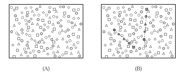
Figure 1: The linkage problem is to find one point at each time step such that the points fit the model for a candidate track. Points from each of the five different time steps are shown as different shapes (square → circle → triangle → diamond → plus). Two linear linkages are shown (B) and a third is left as an exercise for the reader.

This is an important problem in such fields as target tracking and computer vision, but our primary motivating example in this paper is the asteroid linkage problem. Here we wish to determine which observed objects correspond to the same true underlying object from a series of visual observations of the night sky. These linkages can then be used to determine tentative orbits, attribute the observations to a known orbit, and assess the potential risk of an asteroid. The use of new observation techniques and equipment has increased the scope and accuracy of this problem, providing the potential to track hundreds of thousands of asteroids. The next generation of sky surveys, such as PanSTARRS or LSST, are designed to provide vast amounts of observational data that can be used to search for potentially hazardous asteroids. Further, these surveys have the potential to allow us to detect and track fainter objects. However, these improvements greatly increase the combinatorics of the problem reinforcing the need for tractable algorithms.

Below we introduce a new methodology for track initiation. Instead of treating track initiation as a sequential decision problem, we exhaustively consider all possible linkages. Thus we provide an exact algorithm for linkages. We then introduce a multiple tree algorithm for tractably finding the linkages. We compare this approach to an adapted version of multiple hypothesis tracking using spatial data structures and show how the use of multiple trees can provide a significant benefit.

2. Problem Definition

The track initiation problem consists of taking sets of observations from different time steps and linking together those observations that fit a desired model without initial estimates of the track parameters. Figure 2 shows a simple one dimensional example with five time steps and a linear model. The sets of linked observations are shown as open circles with their linear models as dashed lines.

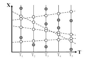
Figure 2: A set of one dimensional observations linked together by linear tracks. The white circles are the observations that correspond to the linear tracks (dashed lines).

Formally the linkage problem can be phrased as a filtering problem. At each time step k we observe Nk points from both the underlying set of tracks and noise. Given a set of observations at K distinct time steps, we want to return all tuples of observations such that:
1. the tuple contains exactly one observation per time step, and
2. it is possible for a single track to exist that passes within given thresholds of each observation.

Thus we wish to filter the ∏ Kk =1 Nk possible tuples down to just those tuples that could be feasible tracks.

The observations consist of real-valued coordinates in D dimensional space, with x i indicating the i th observation. These coordinates are the dependent variables of the track. We use ti to indicate the independent variable of the i th observation. Although in many of the applications below ti will correspond to the time of the observation, it can be used to represent any independent variable.

The second condition specifies a constraint on the observations’ fit to the underlying model. A tuple of observations (x I 1, ···, x IK) is valid only if there exists a track g such that:

δ L [ d ] ≤ x Ii [ d ] − g (tIi)[ d ] ≤ δ H [ d ] ∀ d, i (1)

Equation 1 states that a track g is feasible for a tuple of observations if it falls within some bounds [ g (tIi)[ d ]+ δ L [ d ], g (tIi)[ d ]+ δ H [ d ]] of each observation x Ii in each dimension d. The thresholds δ L and δ H provide upper lower bounds on the fit. Figure 3 shows an example of a feasible triplet using linear tracks and one feasible track for these points. The track is allowed to pass anywhere within the error bars around each point.

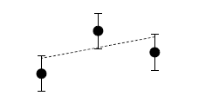
Figure 3: Three points that are compatible for linear tracks.

The above definition of feasibility is compatible with a range of statistical noise models. For example, we can define an arbitrary observation noise model for the points on a track and set the thresholds in each dimension to be the 95% confidence interval for the noise in this dimension. Figure 4 shows an example of this. Further, we can vary δ L and δ H to account for systematic or time varying errors.

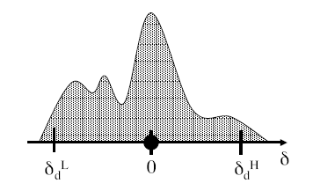
Figure 4: An arbitrary probability distribution and the resulting bounds. The circle denotes the observed location and the upper and lower bars indicate the acceptable locations for the track.

In contrast to the flexibility for noise models, it should be noted that the above criteria does not allow for a concept known as process noise. This means that we assume the track always follows the model. For example, a linear track model cannot account for changes in velocity. This is briefly discussed in Section 8.

Our discussion below focuses on two major types of tracks: linear and quadratic. The quadratic track is simply a quadric function of time:

g (t) = a · t ² + b · t + c (2)

and can be used to describe physical motions of objects undergoing constant acceleration. The linear track is a linear function of time:

g (t) = b · t + c (3)

and can be used to describe the physical motion of objects traveling at a constant velocity. In addition, the linear model can be used for such queries as finding lines or edges described by the observations. While much of our discussion and techniques presented below will also apply to other track models, we restrict the discussion to the linear and quadratic models to keep the discussion simple and consistent.

3. Previous Work

There are a variety of different approaches to the problem of track initiation. Below we briefly discuss some of the more common ones. These approaches differ from our own in several important ways. First, we are asking a different type of query. Specifically, we are asking for all sets of observations that could feasibly belong to a path. Second, we provide an exact algorithm for answering this query.

3.1 Sequential Track Initiation

One common approach to track initiation is sequential track initiation [Blackman and Popoli, 1999]. The unassociated points are treated as new tracks and projected to the later time steps where they are associated with other points to form longer tracks. There are many variations to this type of approach. One common and often successful variation is a very simple form of multiple hypothesis tracking. When a tentative track matches multiple observations at a given time step, multiple hypothesizes (tentative tracks) are formed and the decision is delayed to a later time step. This process is illustrated in Figure 5. The single point matches three other points at the second time step. These points are used to create three hypothesized tracks. This process continues to the third and fourth time step with “bad” hypotheses being pruned away.

In order to reduce the number of candidate neighbors examined gating is used. As shown in Figure 6, neighbors are first filtered by whether they fall within a window or gate around the track’s predicted position. This approach has also been used in conjunction with kd-tree structures to quickly retrieve the candidate observations near the predicted position of a track [Uhlmann, 1992, Uhlmann, 2001 ].

There are several potential disadvantages of this type of approach that arise from the sequential nature of the search itself. It does not use evidence from later time steps to aid early decisions. Early “good pairs” may be easily pruned using a lack of further points along the track. Further, this approach has the potential of being thrown off by noise early in the track. Multiple hypothesis tracking attempts to mitigate this problem by allowing multiple tentative tracks, but introduces another problem, the possibility of a high branching factor causing a significant computational load.

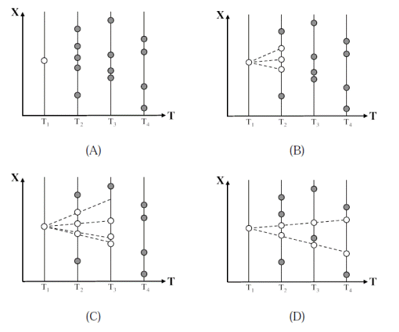
Figure 5: A multiple hypothesis tracker starts from a tentative track (A) and sequentially checks the later time steps. If multiple points fit a candidate track then several hypothesis are created (B) and (C).

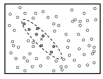
Figure 6: Gating can be used to ignore points that could not be part of the current track. The predicted position of the track is shown as an X and the points that fall within the gate are shaded.

It should be noted that sequential track initiation has the advantage that it can be applied to multiple tracks simultaneously. This gives this approach the ability to discount observations that are “obviously” members of other tracks.

Figure 7: Early noise in a track can significantly throw-off predicted positions. The true points are shown as open circles and the observed points are shown as shaded circles.

3.2 Parameter Space Methods

Another approach to the problem of track initiation is to search for tracks in parameter space. One popular algorithm is the Hough transform [Hough, 1959]. The idea behind these approaches is that for many simple models, individual observations correspond to simple regions or curves in parameter space. An example with a linear model is shown in Figure 8. The points are shown in Figure 8.A and their corresponding lines in parameter space in Figure 8.B. If a series of observations lie along a line, then their lines in parameter space will intersect at a common point. The Hough transform looks for lines by using grid-based counts of the number of lines that go through a particular region of parameter space (Figure 8.C and 8.D).

There are several major downsides to the parameter space approach. First, maintaining and querying the parameter space representation can be expensive in terms of both computation and memory. There are many possible intersections to check and storing occurrences in a grid structure may require significant amounts of space. Secondly, the level of discretization of parameter space can drastically affect the accuracy of the algorithm.

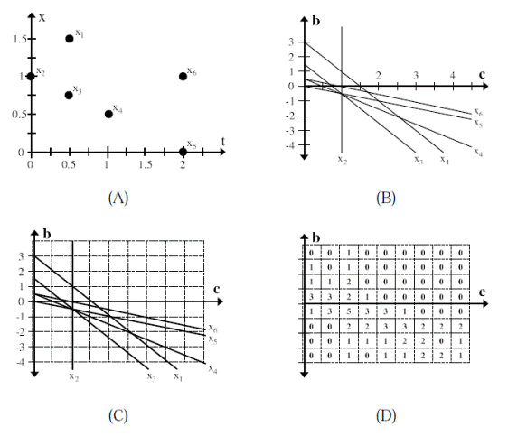
Figure 8.

If the grid is too tight then a small amount of noise can cause intersections to spread out over several bins and be missed. If the grid is too loose then coincidental occurrences can accumulate and cause false alarms. Although the false alarms can be filtered out in post-processing, this step further increases the computational cost.