Laplace transform

Lecture 1.4b

Laplace transform

Laplace transform table

Properties of the Laplace transform

Inverse Laplace transform and Common partial fraction expansions

Graphical evaluation of the residues

Test input signals

- step function

- -function

- the connection between the step and impulse response

- harmonic (sine-shaped) input signal

- ramp (linear increasing) input signal

- quadratic (parabolic) time function and others.

Laplace transform

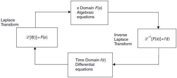
In order to compute the time response of a dynamic system, it is necessary to solve the differential equations (system mathematical model) for given inputs. There are a number of analytical and numerical techniques available to do this, but the one favored by control engineers is the use of the Laplace transform.

This technique transforms the problem from the time (or t) domain to the Laplace (or s) domain. The advantage in doing this is that complex time domain differential equations become relatively simple s domain algebraic equations. When a suitable solution is arrived at, it is inverse transformed back to the time domain. The process is shown in Figure 4.1.

The Laplace transform of a function of time f(t) is given by the integral

(4.1)

Where s is a complex variable () and is called the Laplace operator.