FIGURE 4.2 (a) Spring-mass-damper system. (b) Free-body diagram.

To illustrate the usefulness of the Laplace transformation and the steps involved in the system analysis, reconsider the spring-mass-damper system being studied by you earlier described by Equation (3.1), which is

(4.16)

We wish to obtain the response, y, as a function of time. The Laplace transform of Equation (4.16) is

(4.17)

Left and Right Limits:

Left Hand Limit:
Let 'a' be any fixed point. If 'x' approaches to 'a' through the value of 'x' less than 'a'. Then the limit is called left hand limit.
Thus, limit is denoted by

Right Hand Limit:
Let 'a' be any fixed point. If 'x' approaches to 'a' through the values of 'x' greater than 'a'. Then the limit is called right hand limit.
Thus, limit is denoted by

When , and , and

we have

(4.18)

Solving for Y(s), we obtain

(4.19)

The denominator polynomial q(s), when set equal to zero, is called the characteristic

equation because the roots of this equation determine the character of the time response. The roots of this characteristic equation are also called the poles of the system.

The roots of the numerator polynomial p(s) are called the zeros of the system; for example, is a zero of Equation (4.19). Poles and zeros are critical frequencies.

At the poles, the function Y(s) becomes infinite, whereas at the zeros, the function becomes zero. The complex frequency s -plane plot of the poles and zeros graphically portrays the character of the natural transient response of the system.

For a specific case, consider the system when k/M = 2 and b/M = 3. Then Equation (4.19) becomes

(4.20)

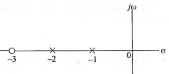
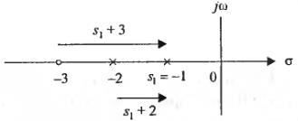
FIGURE 4.3 An S -plane pole and zero plot.

	= pole
	= zero

The poles and zeros of Y(s) are shown on the s-plane in Figure 2.

Expanding Equation (4.20) in a partial fraction expansion, we obtain

(4.21)

where and are the coefficients of the expansion. The coefficients are called residues and are evaluated by multiplying through by the denominator factor of Equation (4.21) corresponding to and setting s equal to the root. Evaluating when = 1, we have

(4.22)

and = -1. Alternatively, the residues of Y(s) at the respective poles may be evaluated graphically on the S-plane plot, since Equation (1.22) may be written as

(4.23)